Scenario
Now that we’ve had our first look at AWS Glue DataBrew, it’s time to try it out with a real data preparation activity. After nearly a year of COVId-19, and several rounds of financial relief, one interesting dataset is that from the SBA’s Paycheck Protection Program (PPP). As with al government programs, there is a great deal of interest in how the money was allocated. The PPP was a decentralized program, with local banks approving and disbursing funds. The loan data for the program was released in several batches, and early indication is that the data is a bit of a mess, making it difficult for groups without a data prep organization to analyze the data. As data professionals, we can help with that.
Setup
The link to the most recent PPP data is available is found at https://www.sba.gov/funding-programs/loans/coronavirus-relief-options/paycheck-protection-program/ppp-data. I downloaded the Nov 24, 2020 dataset, and uploaded the files to an S3 bucket.
Our work with DataBrew begins, as many things in AWS do, by creating a service level IAM role and granting permission to our data, as documented at https://docs.aws.amazon.com/databrew/latest/dg/setting-up-iam.html.
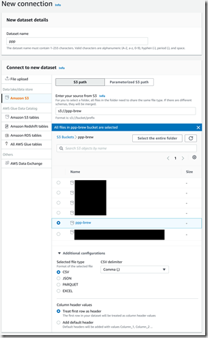
After we’ve uploaded our data and given DataBrew permission, it’s time to create a Dataset, which is basically a pointer to the data files we’ll be using. We’ll need a Dataset for every different batch of data we want to use.
Initial Profiling
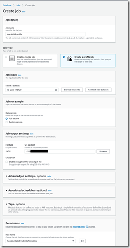
The first thing I like to do when I get an unknown dataset is profile as much of the data as I can. With DataBrew, I can easily set up a Profile Job to gather statistics about the entire dataset. To start, we navigate Jobs >> Profile Jobs >> Create Job. The configuration looks like the image below.
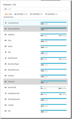
The profiling job takes a little over one minute to run since DataBrew will profile a maximum of 20,000 rows even if you select “Full dataset” (you can request a limit increase). Once complete, we can choose to “View data profile”, then the “Column Statistics” tab to check for completeness, type and validity.
Most of the columns are 100% valid, which would be fantastic if true, although I suspect unknown values may be represented by a value which DataBrew does not recognize as “unknown” or “invalid”. We’ll need to investigate further. Also, ZIP Code was identified as a numeric column, which is a very common mistake made by data profilers. Many US Zip Codes start with zero, and need to be treated as strings in order to retain that leading zero.
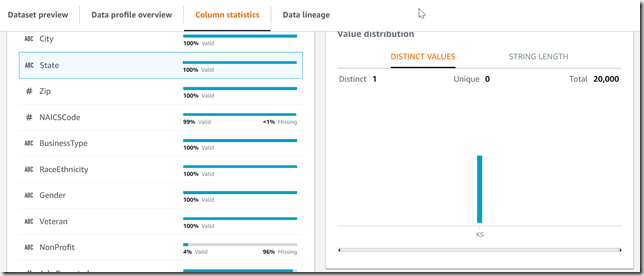
State claims to be 100% valid, so let’s take a look at the values. Of the 20,000 records profiled, all were in Kansas. Deep sigh. We’re going to need to try a random sample somehow.
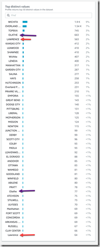
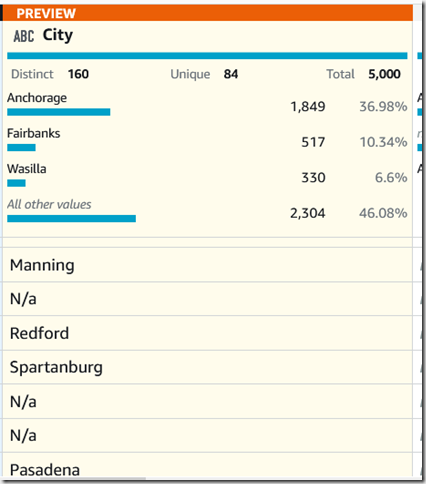
Cities are where the fun usually begins, and looking at the Top 50 values, we see that there is inconsistent casing and DataBrew treats “OLATHE” and “Olathe” differently. We see the same treatment with “LAWRENCE” and “Lawrence”, too. That’s something we can try and fix in our data prep. Trivia note: “Pittsburg” is spelled correctly here, only Pittsburgh, PA has the “h” at the end.
Random Sampling
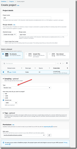
That’s a good start, but let’s see what else we can find with a random sample. To do a random sample, we need to create a project, using the same dataset, and configure the sampling to be 5000 random rows.
After the sampling is complete, we’re taken to the projects tab, where we can review the sampled data. Right away we can see that “Not Available” and “N/A” are very common answers, and we need to work with our business partners to decide if these are values we want to count, values we want to convert to a different value, or if we want to count them as invalid results.
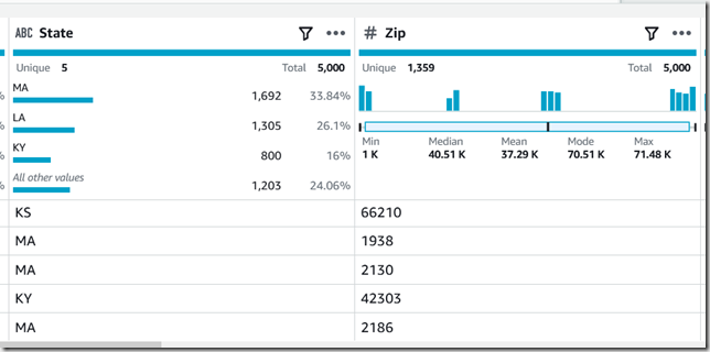
Looking at some of the ZIP Codes, we can see that the column was profiled as a number, and some of the MA ZIP Codes lost their leading 0. We’ll need to change the column type and put the leading 0 back using a transformation.
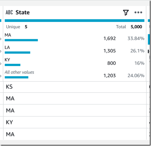
Looking at the State column, the random sampling did improve the sample somewhat—we now have 5 states represented instead of just one.
Recipe
Now that we have a couple columns which need a transformation, and a decent random sample, it’s time to start create our first recipe. We’ll clean up both the ZIP Code and City name column and let our business users work with the data while we look for some additional transformations.
ZIP Code
Since ZIP Code was incorrectly typed as a numeric column, we need to correct this before we produce an output for our users. This means we need to re-type the column as a string and pad the leading zero where it was stripped off.
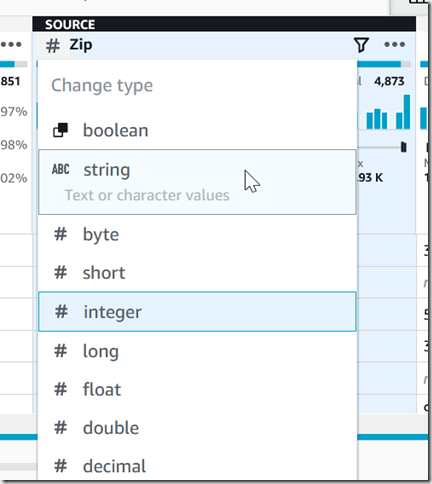
To change the type of the column, click on the “#” next to the column name and choose “string”. This will add a recipe step to convert the type of this column, but will not replace the leading zero.
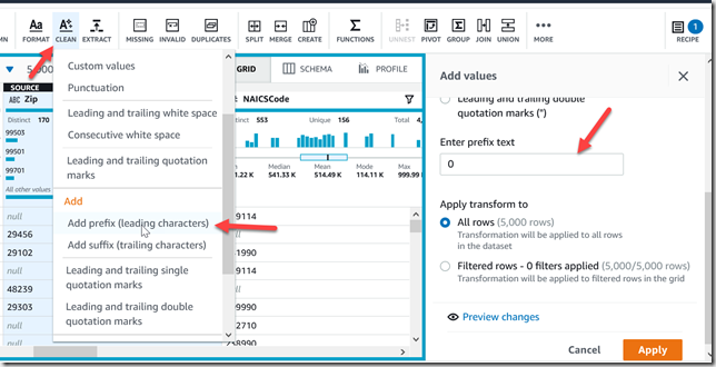
In order to replace the leading 0, we can rely on the old trick of prefixing every value with a 0 and take the right five characters to create the full zip code. This is a two-step process in our recipe. First, we pad all values with 0 by activating the Clean menu, selecting “Add prefix…”, then entering a prefix text of 0.
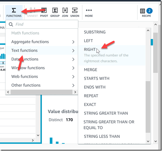
This prefixing will be applied to all values, which will make most ZIP Codes six characters long. To fix this, we take the right five characters by activating the Functions menu, selecting Text Functions, then Right.
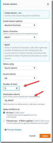
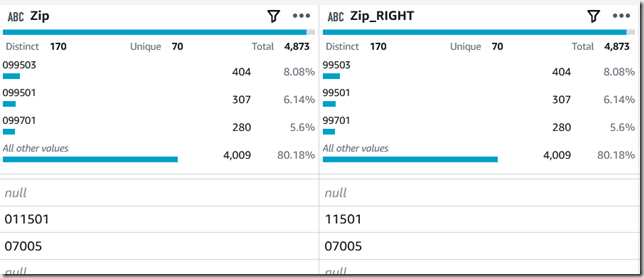
This operation will create a new column, which by default is labeled “Zip_RIGHT”, and we configure the number of characters to keep.
And when we preview the change, this is how it looks.
City
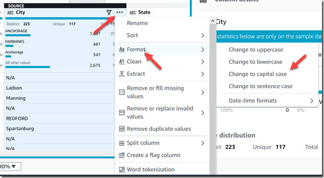
As we saw in the profile results, city names are both mixed case and all uppercase, which is causing mis-counts by city. We need to standardize the capitalization to alleviate this. For our needs, it doesn’t matter if we use all uppercase or not, just as long as we’re consistent. I’ll use proper case because it doesn’t look like I’m being yelled at. We can either activate the Format menu (either from the menu bar or using the ellipses menu) then choosing “Change to capital case”.
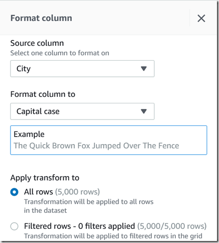
We can then see an example of what each formatting option will do. Capital case is the closest option for how most city names are capitalized. It’s not perfect, but it’s consistent, and we’d need an address verification system to do better. This option changes the value in the original column, it does not create a new column.
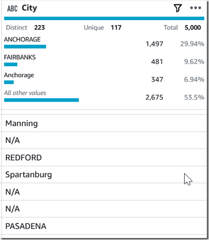
We can even preview the changes, and see how ANCHORAGE and Anchorage are now combined into a single value of Anchorage.
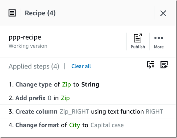
Our recipe now looks like this, which is good enough for now.
Publishing and Using the Recipe
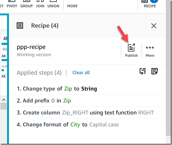
In order to run this recipe against the full dataset, or to run it again, we need to publish it and then create a Job. From the Recipe panel, we click the Publish button. Recipes are versioned, so in the pop-up we add some version notes and Publish. Once Published, we can use it in a Job.
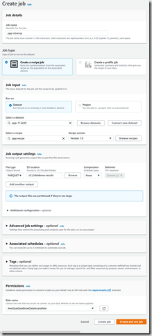
I covered Jobs in detail in the First Look: AWS Glue DataBrew, so here is how I configured the job:
Parquet is a great storage format, it has a schema, it’s compact, columnar for performant query, and it’s native to many of AWS’s services. Once the job has completed, how do we ensure it worked? Simple, we use the output as a new Dataset and profile the results. Viewing the results of the profile of the cleanup job, we can see the top 50 City names are all capital case.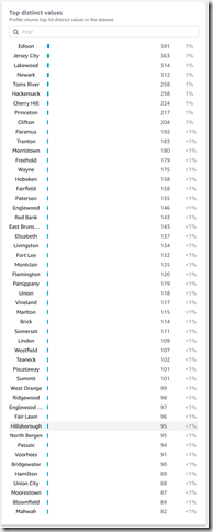
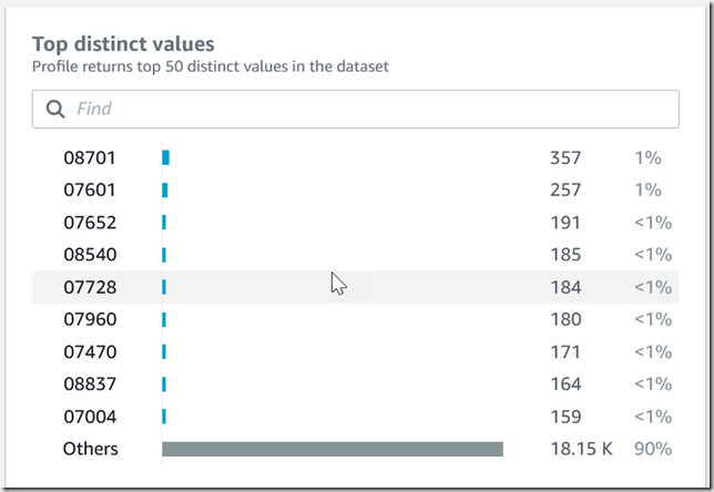
Similarly, we can see the ZIP Codes are all 5 characters long and have the leading zero (fortunately, the profile job sampled New Jersey).
Congratulations, we can now start to make this data available to our users! We know they’ll find more steps we need to add to our recipe as they begin to work with the data, but this is a great start. Find me on Twitter @rj_dudley and let me know how you find DataBrew.
