rjdudley

15 S3 Facts for S3’s 15th

To celebrate S3’s 15^th birthday on 3/14/2021, and to kick off AWS Pi Week, I tweeted out 15 facts about S3. Here they are as a blog post, to make them easier to read. Because of the rapid pace of innovation in AWS services, including S3, so if you’re reading this in the future, some things may have changed.

1. S3 is designed for “eleven 9s” of durability. When you take into account redundancy in and across availability zones, in 10,000,000 years you’d lose only lose one of 10,000 objects. Read more at https://aws.amazon.com/blogs/aws/new-amazon-s3-reduced-redundancy-storage-rrs/.

2. S3 is region-bound, which means all S3 buckets in that region are partying in the same publicly available cloud ether. You can restrict access to a VPC but the bucket is still located outside the VPC. Related: https://cloudonaut.io/does-your-vpc-endpoint-allow-access-to-half-of-the-internet/.

3. S3 is a very versatile storage service. The trillions of objects it stores are the basis for many workloads, including serving websites, video streaming and analytics.

4. The return of INI files! With a first byte latency of milliseconds, S3 is suitable for storing configuration settings in an available and inexpensive way. Databases are no longer a fixed cost and there is no need for one just for configuration.

5. S3 is designed for “infinite storage”. Each object can be up to 5TB in size, and there is no limit to the number of objects you can store in a bucket. Analytics aren’t constrained by a file or disk size. It’s like a TARDIS, or bag of holding!

6. How do you perform operations on hundreds, thousands or more objects? S3 Batch Operations allow you to copy objects, restore from Glacier, or even call a lambda for each file. For more information, see https://aws.amazon.com/blogs/aws/new-amazon-s3-batch-operations/.

7. S3 is a “consumption model”, so you pay only for what you use when you use it. No more provisioning fixed-size network storage solutions with large up-front costs.

8. But what if you need massive object storage closer to your location? S3 on Outposts puts S3 on-premises, right where you collect or process your data. For more info, start at https://aws.amazon.com/s3/outposts/.

9. If your bandwidth is limited or non-existent, you can use Snowball Data Transfer to move TB to PB of data in and out of AWS. Learn more at https://aws.amazon.com/snowball/.

10. For data collection and object generation at the most extreme edges there is Snowball Edge Storage. Snowball Edge can even run processing workloads. Read more at https://docs.aws.amazon.com/snowball/latest/developer-guide/whatisedge.html.

11. Although you can upload files to S3 via the console, CLI and REST API, wouldn’t it be great if you could just drag a file to a network share and have it appear in the cloud? With a File Gateway, you can do exactly that! See https://aws.amazon.com/storagegateway/file/.

12. S3 offers multiple storage classes, so you can optimize cost, latency and retention period. Standard offers the lowest latency but at the highest cost, while Glacier Deep Archive is perfect for yearslong retention. Read more at https://aws.amazon.com/s3/storage-classes/.

13. S3 Storage Lens is a central dashboard organizations can use for insight into S3 utilization and to get recommendation to optimize price. Read more at https://aws.amazon.com/blogs/aws/s3-storage-lens/.

14. S3 can version objects, so if you accidentally delete or profoundly update an object, you can recover from the most recent save or many prior versions, too.

15. S3 is a very secure service. IAM policies can be applied at the bucket and object level with a great deal of granularity. Additionally, VPC endpoints bind S3 traffic to a specific VPC only.

And one to grow on (for everyone): AWS recently released three new S3 training courses: https://aws.amazon.com/about-aws/whats-new/2021/01/announcing-three-new-digital-courses-for-amazon-s3/.

First Look: AWS Glue DataBrew

Introduction

This is a post about a new vendor service which blew up a blog series I had planned, and I’m not mad. With a greater reliance on data science comes a greater emphasis on data engineering, and I had planned a blog series about building a pipeline with AWS services. That all changed when AWS released DataBrew, which is a managed data profiling and preparation service. The announcement is at https://aws.amazon.com/blogs/aws/announcing-aws-glue-databrew-a-visual-data-preparation-tool-that-helps-you-clean-and-normalize-data-faster/, but the main thing to know is that DataBrew is a visual tool for analyzing and preparing datasets. It’s powerful without a lot of programming. Despite its ease of use and numerous capabilities, DataBrew will not replace data engineers; instead, DataBrew will make it easier to set up and perform a great deal of the simple, rote data preparation activities, freeing data engineers to focus on the really hard problems. We’ll look into use cases and capabilities in future blog posts. Spoiler alert: we’re still going to need that pipeline I was going to write about, just more streamlined. Updated series in future posts.

DataBrew is not a stand-alone component, but is instead a component of AWS Glue. This makes sense, since it adds a lot of missing capabilities into Glue, but can also take advantage of Glue’s job scheduling and workflows. Some of what I was planning to write involved Glue anyway, so this is convenient for me.

In this “First Look” post I’m working my way through the DataBrew screens as you first encounter them, so if you have an AWS account, it might be useful to open DataBrew and move through the screens as you read. No worries if you don’t, I’ll cover features more in-depth as I work through future posts.

DataBrew Overview

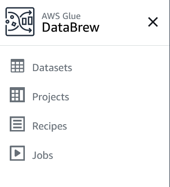
There are four main parts of DataBrew: Datasets, Projects, Recipes and Jobs. These are just where we start, there is a lot of ground to cover.

DataBrew parts

Datasets

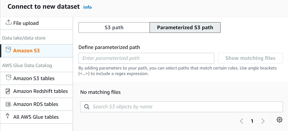
DataBrew can work directly with files stored in S3, or via the Glue catalog to access data in S3, RedShift or RDS. If you’re using Lake Formation, it appears DataBrew (since it is part of Glue) will honor the AuthN (“authorization”) configuration. Exactly how this works is a topic for future exploration.

If you’re connecting directly to S3, DataBrew can work with CSV, parquet, and JSON files. At the time of writing, XML is not supported so you’d need to do a conversion upstream in a Lambda or Spark job. One cool feature is the ability to create parameterized paths to S3, even using a regex. This isn’t something available in the Glue Catalog, only directly to S3. I work with a lot of files which have a date stamp as part of the filename, so this will be helpful.

DataBrew datasets

Projects

Holey moley there’s a lot of stuff here! The Projects screen is where the real action is, and we’ll spend a lot of time here in the future.

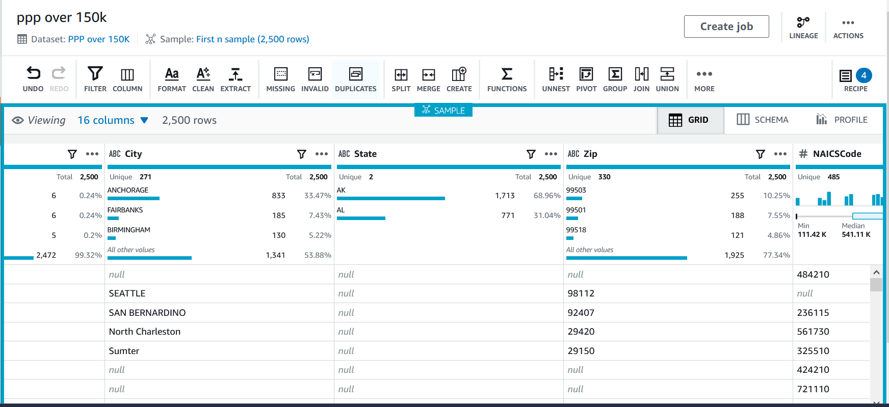
DataBrew Projects

Sample View

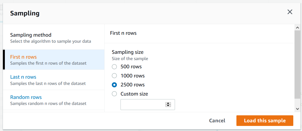
As we explore the Sample View, it’s important to keep in mind that DataBrew is meant for actual data preparation work, not just lightweight profiles. This sample view is kept to a small windows so we can explore the effects of transformations and monitor effects on quality.

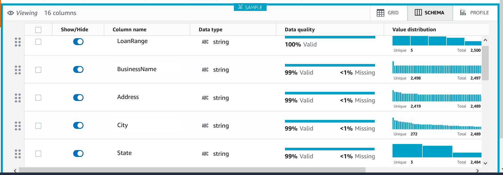
The majority of this page is taken up with a sample of the dataset and some lightweight profiling, including the type, number of unique values in the sample, the most common values in the sample, and the first few rows of the sample. The sample size and position in the set can be changed. This sample view is a great way to test transformations and enrichments, which we’ll look into later.

DataBrew Sample

The profile view can be changed to explore the schema, which will be inferred from CSV and JSON files, or use the metadata in parquet or Glue Catalog.

DataBrew Schema

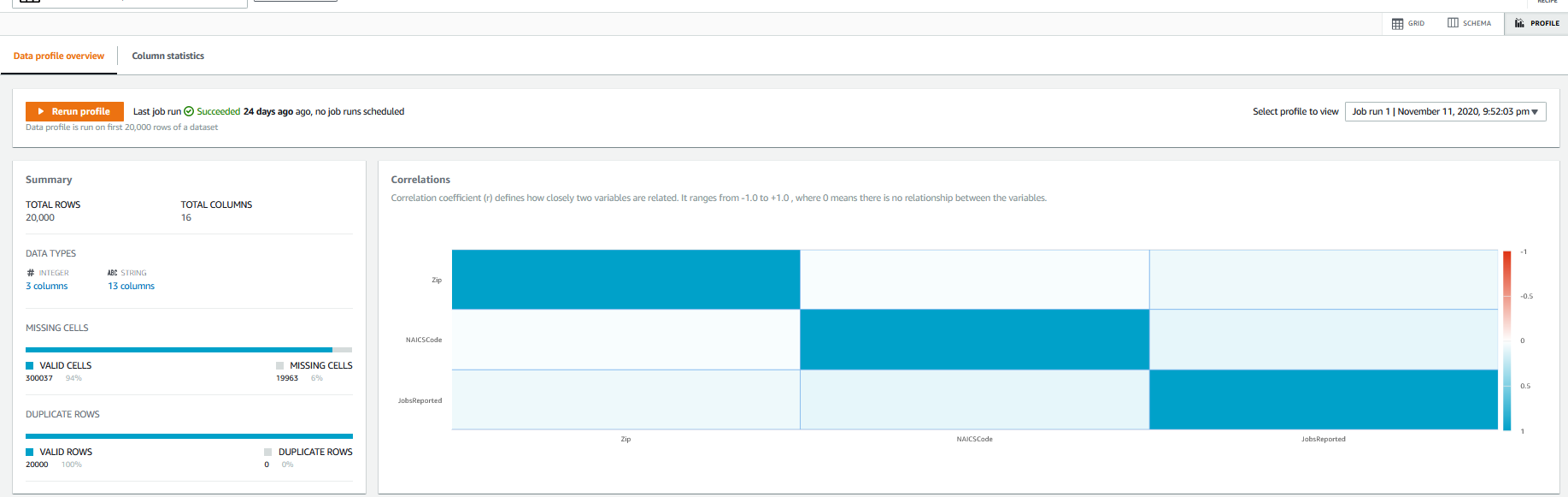
he third profile view is correlations and summaries. If you’ve runs several profiles, the history is available to browse. The “missing cells” statistic is something we will revisit for the dataset I have loaded here. Also, for my sample dataset, the Correlation isn’t that interesting because the majority of the columns are part of an address so they should correlate. But in other datasets, this could be really interesting.

DataBrew Profile Overview

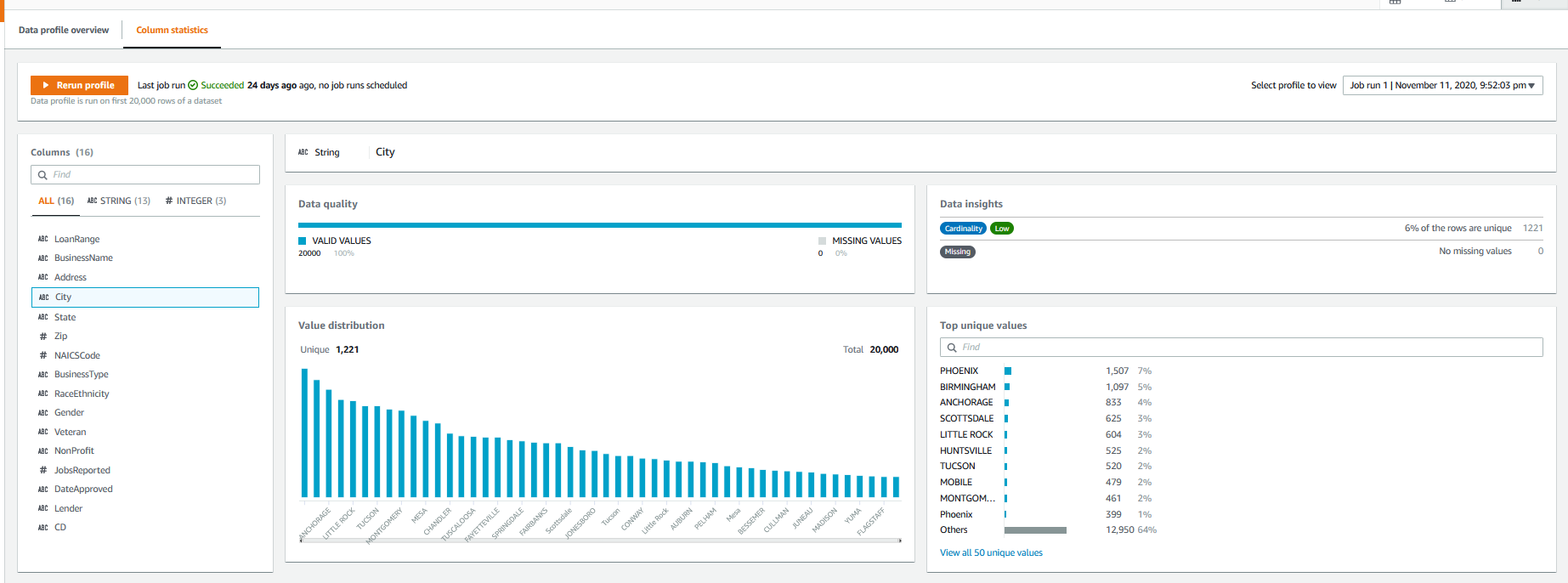
The profile view also has data insights into individual columns, showing several quality metrics for the selected column.

DataBrew Column Stats

Transformations

DataBrew currently has over 250 built-in transformations, which AWS confusingly calls “Recipe actions” in parts of its documentation.

DataBrew Transformations

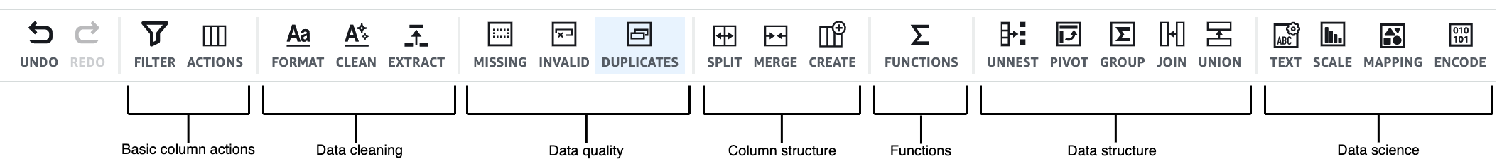
The transformations are categorized in the menu bar above the profile grid. Transformations include removing invalid values, remove nulls, flag column, replace values, joins, aggregates, splits, etc. Most of these should be familiar to a data professional. With a join you can enrich one dataset by joining to other datasets.

Recipes

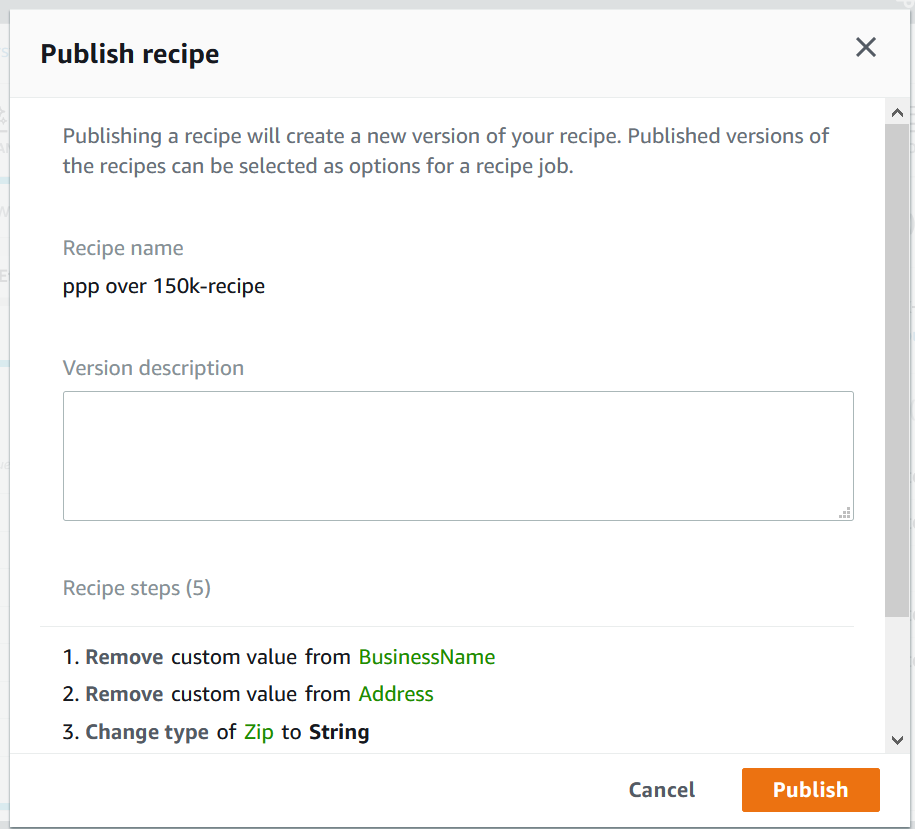
When we’re in the Projects tab, and we apply a transformation to a column, we’re creating a recipe step. One or more recipe steps form a recipe, and there isn’t a published maximum number of recipes per dataset. Since each recipe can be called by a separate job, this provides a great deal of flexibility in our data prep processes. Recipe steps can only be edited on the Projects tab; the Recipes tab lists the existing recipes, allows for downloading of recipes and some other administrative tasks. Recipes can be downloaded and published via CloudFront or the CLI, providing a rudimentary sharing ability across datasets.

DataBrew Recipes Tab

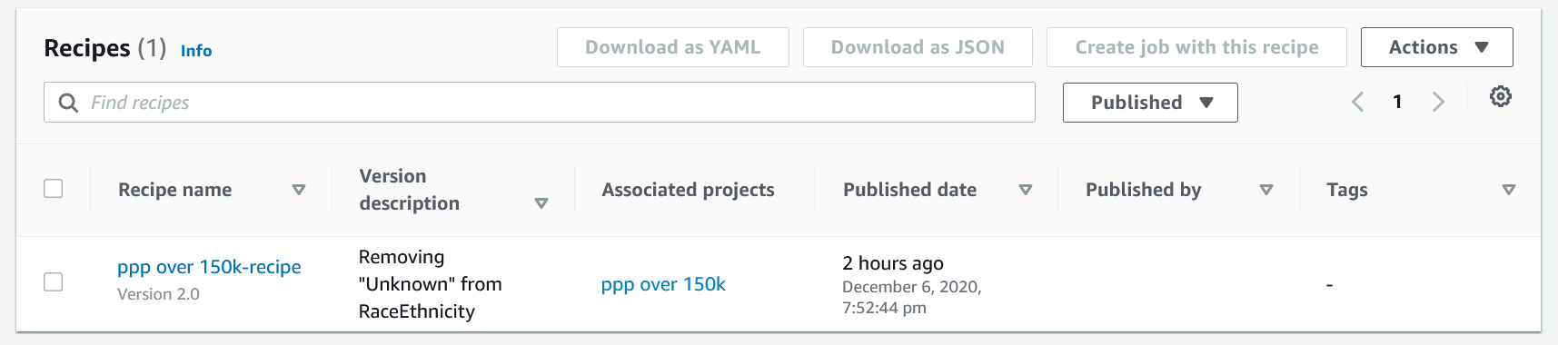
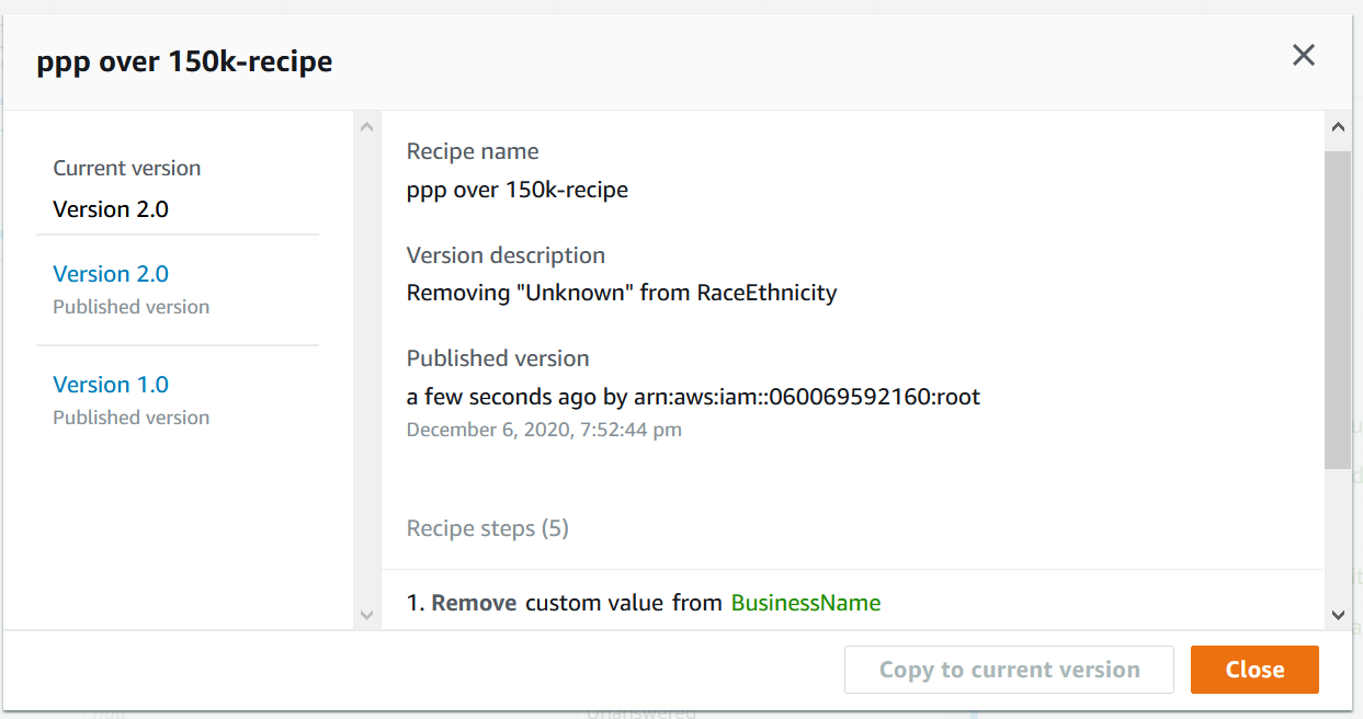
Opening a recipe brings up summaries of the recipe’s versions, and the other tab on this page opens up the data lineage for the recipe. This lineage is not the data lineage through your enterprise, just the pathway through the recipe. My simple example here isn’t that impressive, but if you build a more complex flow with joins to other datasets and more recipes, this will be a nice view. Although you can preview the datasets and recipes at the various steps, this is not a graphical workflow editor.

DataBrew Lineage

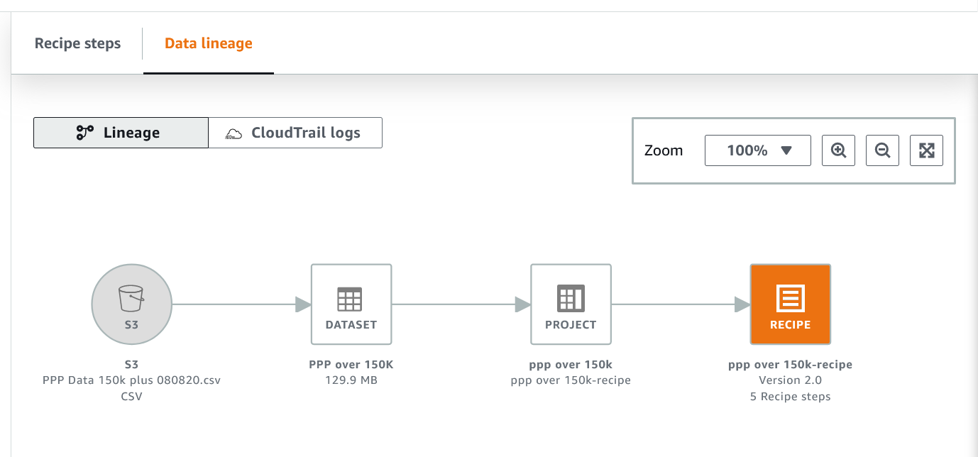
This is also a convenient screen to access CloudTrail logs for the recipes

Jobs

There are two types of jobs in DataBrew–“recipe” and “profile”.

DataBrew Job Types

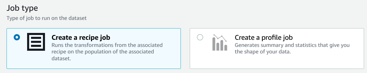
A profile job examines up to 20,000 rows of data (more if you request an increase). The results of a profiling job include:

data type
unique values count
missing values count
most common values and occurrences
minimum and maximum values with occurrences
percentiles, means, standard deviation, median
and more…

One feature missing in the Profiling is determining the pattern or length of text values. The Profiling results are saved in JSON format, can be saved in S3, and there is an option to create a QuickSight dataset for reporting. Anything more than QuickSight will require some custom processing of the JSON output. Although it took this long in a blog post to discuss profiling jobs, a profile is something which really should be created before building recipes.

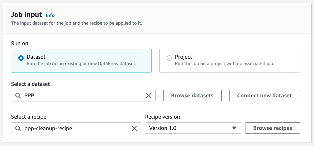
A recipe job configures a published recipe to be run against a selected dataset. In a Dataset job we choose the dataset, recipe and recipe version we want to use.

DataBrew Dataset Job

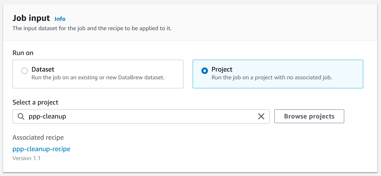
The other recipe job option is is a Project job, which uses a saved project defined on the Projects tab. In this job, the only thing we need to configure is the project.

DataBrew Project Job

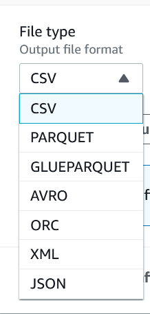
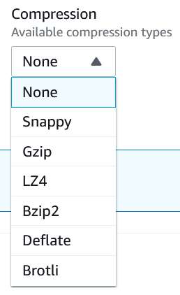
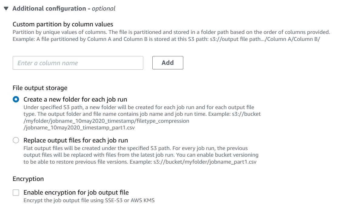
The original dataset is not modified in DataBrew; instead, we configure the S3 location, output file format, and compression for storing the results.

DataBrew Output File Type DataBrew Output Compression

The output can be partitioned on a particuar column, and we can choose whether to overrite the files from the previous run or keep each run’s files. Please use encryption.

DataBrew Output Partitioning

Once configured, jobs can be scheduled. You can have a maximum of two schedules per job. If you need more than two schedules you’ll need to create an identical job.

DataBrew Job Schedule

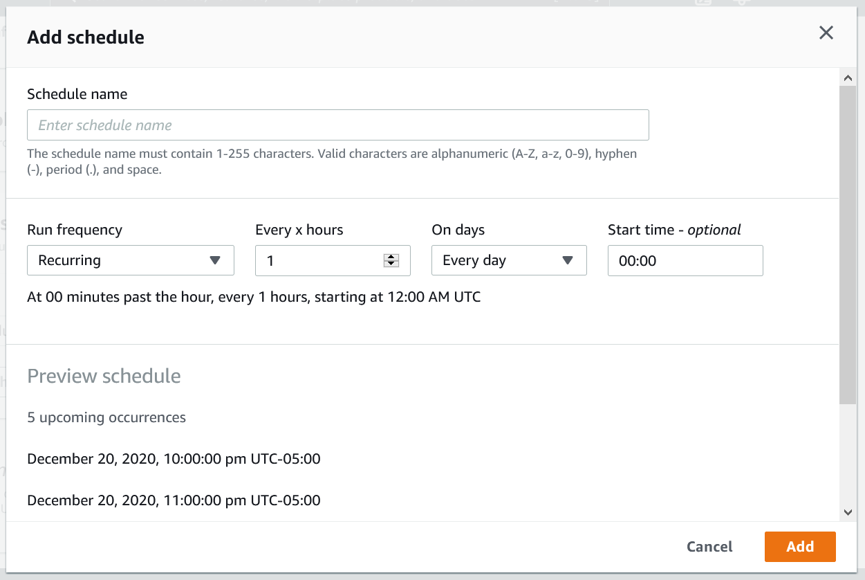
Either type of job can be run on a schedule, on-demand or as part of other workflows (see “Jobs Integrations” below). There is only one recipe and one dataset per job, so processing multiple recipes and/or multiple datasets would require additional workflow.

Jobs Integrations

Aside from the console or a schedule, how else can a DataBrew job be started? For starters, the DataBrew API exposes all the functionality in the console, including running a job. When coupled with lambdas, this exposes a great amount of flexibility in starting a job.

A second option is to use a Jupyter notebook (vanilla Jupyter, not SageMaker notebook yet) and the plugin found at https://github.com/aws/aws-glue-databrew-jupyter-extension.

Source Control Integration

Recipes and jobs have a form of versioning, but it seems to be S3 object versioning since there isn’t a real source control workflow, but rather a new version is created with every published update.

DataBrew Publish Recipe

DataBrew Recipe Versions

However, as with most of AWS’s online editors, there is no direct source control integration. The best you can do is to download recipes and jobs as JSON and check them in manually. Better than nothing but still surprising since AWS has CodeCommit.

Infrastructure as Code

At this time, neither Terraform nor Pulumi support DataBrew, but CloudFormation can be used to script DataBrew; see the https://docs.aws.amazon.com/AWSCloudFormation/latest/UserGuide/AWS_DataBrew.html for the API documentation and examples. The CLI is another scripting option, the documentation for the CLI is at https://awscli.amazonaws.com/v2/documentation/api/latest/reference/databrew/index.html.

Cloud Native AWS Development On A Chromebook Using VS Code

Whew! That’s a lot to unpack there. Let’s start in the middle, with the Chromebook, They’re not widely known as development machines. They are limited in RAM, persistent storage and processor speed. The OS has limited application support, especially for ones which rely on arbitray code execution like most IDEs. They have great battery life, small size, and are usually easy to procure (exept in the current return to school COVID shortage).

The newer Chromebooks (see https://sites.google.com/a/chromium.org/dev/chromium-os/chrome-os-systems-supporting-linux for a list of supported devices) have an interesting beta feature–the ability to install a Linux virtual machine. Termed Crostini, this is a supported way to install a Linux distro (Debian stretch). This opens up all kinds of possibilities, especially since the user’s home folder of the VM is mounted as local storage in the Chrome OS.

Microsoft’s VS Code is a fantastic free cross-platform code editor, and can be installed via the Linux command line. Not to give away any spoilers, but VS Code (and its extensions) runs seamlessly as if it is a native application even though it’s installed in the Linux VM. There is a rich ecosystem of extensions, a few of which will be useful for us.

Ckoud native development is more like infrstructure configuration and control; the definition is closer to “we’re connecting and orchestrating AWS’s services, rather than coding everything from scratch”. This is why you sometimes hear the term “infrastructure as code” (IAC)–we use a configuration language to write instructions to direct the activities of AWS’s services, then deploy the instructions to the service, and test our IAC. This works in our favor because we can write the code locally and deploy the code via AWS’s command line interface. Fortunately, the AWS CLI tooling can also be installed and run on the Linux VM, giving us a way to deploy our code from a Chromebook. AWS’s infrastructure language is defined using Cloud Formation, and VS Code has several Cloud Formation extensions, including a template library, to facilitate our work. When a custom coded application is needed, the serverless application model is used (the SAM pattern characteristics are small services with an API interface written in a cross-platform language and deployed in a container).

It’s sounding more promising that we can use a Chromebook for AWS development, doesn’t it? One last thing you’ll need–an AWS account, so get one if you don’t have one already. There is a free-tier, and everything I’ll be doing will use services or service limits which should be “free forever”.

Here’s how I set up my development environment. By the way–we’ll be using the Linux command line interface (CLI), which I am still learning also. If you’re not familiar, I’ve found this book to be invaluable: http://linuxcommand.org/.

Install Crostini

The Crostini beta makes this step as simple as enabling the feature and waiting for several minutes. At this time, the VM is loaded on the main drive and consumes a lot of space, so depending on what else you want to do on your machne, you may need to minimize the number of other things you install or save on the main drive.

The installation instructions are at https://support.google.com/chromebook/answer/9145439. Make sure you read the entire page, since there is important information beyond just installation.

After you’re done, make sure to open the Terminal and run “sudo apt-get update” and “sudo apt-get upgrade” to make sure you have the latest patches.

Install VS Code

Here we are in the CLI! Microsoft’s instructions can be found at https://code.visualstudio.com/docs/setup/linux#_debian-and-ubuntu-based-distributions. Crostini is a newer Debian-based distro so it’s only a couple simple steps.

There is an easier way to install, though. You can downoad the .deb package from the official site, then right-click the package and choose “Install with Linux (Beta)” from the menu. The installer will run for a minute or two, and presto! VS Code will be installed.

install VS Code from .deb package

Add CloudFormation Extensions

A moment of truth! Open VS Code, and if it runs, great job! Now it’s time for an extension to make our development easier, the CloudFormation extension, https://marketplace.visualstudio.com/items?itemName=aws-scripting-guy.cform.

CloudFormation instructions are called stacks (plural: stackset), and can be written in either JSON or YAML. Stacks are also difficult to write from scratch correctly. The templates in this extension will make our lives much, much easier.

Install and Configure the AWS CLI v2 for Linux x86

AWS provides us a couple ways to administer its services. You can interact via the web-based console but ultimately we want to get to a higher degree of repeatability and automation in our deployment processes, and the CLI gets us a little closer. Installation instructions are at https://docs.aws.amazon.com/cli/latest/userguide/install-cliv2-linux.html, and configuration is the next section.

Once installation is complete, you can open the Terminal and run “aws –version”. If that works, you’re good to go with configuration. The most important configuration is the access keys the CLI will use to connect to AWS service APIs. Although you can use your root user login, it’s not a good idea. Instead, you should create a new IAM user for the CLI. This is done in the AWS console, and there are a lot of steps in creating a new IAM user, but you can’t really screw anything up. Worst case, delete the user and start over. In step 2 of the wizard (image below) you’re asked to put the new user in a group or attach directly to an IAM profile. For now, it will be easiest if you attach directly to the AdministrativeAccess profile. We can always titrate this down later, but there are 580+ profiles to sort through and we don’t know which ones we need yet.

user wizard step 2

Once your new IAM user is created, you’ll need to follow the configuration for credential file settings at https://docs.aws.amazon.com/cli/latest/userguide/cli-configure-files.html. That’s all we need for now.

Install git

Source control is always a best practice. VS Code, the extensions and the SDKs are all cross platform, so if you install the Windows or Mac bits on another machine, you can easily transfer your code from machine to machine with version history and backup.

Assitionally, we can also use GitHub Actions to deploy our code, but that’s for a future post. I plan to start with the CLI.

Installation for Linuz is found at https://git-scm.com/download/linux.

Notes:

The crouton project may be able to be used to install Ubuntu side-by-side with Chrome OS (see https://ubuntu.com/tutorials/install-ubuntu-on-chromebook#1-overview) but this is not a supported installtion. It would provide a more native Linux experience, though.

Deeper info about Crostini at https://chromium.googlesource.com/chromiumos/docs/+/master/containers_and_vms.md

Feedback? Find me on Twitter at @rj_dudley.

GitHub/BitBucket For The People Who Just Got a Raspberry Pi and Are In Facebook Groups Asking Questions

(work in progress – kids woke up before I was done but I wanted to share what I had, updates will come)

Few things are more awesome than being curious and being able to spend a few bucks on a small board to follow your curiosities. There is a lot of fun ahead, but there are also going to be frustrations. I’ve been a professional software programmer for almost 20 years and I am frequently still stumped. When you hit these times, don’t be discouraged, ask questions and experiment because the success is worth 100 frustrations. I promise you.

I’m writing this because I’m in a couple Raspberry Pi groups on Facebook, and I see questions about better ways to store scripts and save documents every couple of days. If you’ve asked that, your instincts are spot-on, and even if you’ve never written a line of code this instinct alone puts you above about 10% of the people I’ve ever interviewed for a job. It probably also means you’re experimenting with code a bit (experimenting with code is how you get past those frustrations), and you need a better way to keep track of your changes than naming your files “led.py.new.old.old.1.old”. Been there, done that. Let me explain the better way.

BTW – this blog post is meant to complement and explain already available documentation, not replace what exists. So I’ll explain the fundamentals of what you’re doing but link to official documentation.

What are GitHub and Bitbucket?

GitHub and Bitbucket are two commercial services which provide source code management (SCM). This means they’re meant to keep your code files safe and organized, and keep a history of your changes. You can use this history to make something work, commit that working file, then screw it all up on your device trying something new, then be able to retrieve a previous version. Because of the version history, you’ll sometimes hear these called “version control systems”, or just “VCS”.

Both GitHub (GH) and Bitbucket (BB) offer free plans with both public (for sharing) and private (because sometimes my code is embarrassingly bad when I’m tinkering) repositories. They both offer very similar features, either one is a good choice for you, but GitHub is a lot more popular in the open source world. I used Bitbucket for my personal work for a long time, but the popularity of other projects made GitHub my main system now.

Both GH and BB are based on an open source version control system called “git“, which was developed in 2005 by Linus Torvalds to use for developing Linux (see https://en.wikipedia.org/wiki/Git for the rest of the story). GH and BB provide the cloud-based server side of keeping your code safe, you’ll still need something on your computer. The basic git uses the BASH command-line shell on every OS (Linux, Mac, Windows, Raspbian, etc.), but there are also plenty of GUI clients available. Because Rapsbian is derived from the same Linux kernel as Ubuntu, almost anyone which runs on Ubuntu will run on Raspbian. That being said, I really recommend learning the BASH commands so you have a little better understanding of how git works, but also the Raspberry Pi has limited processing and the shell doesn’t take much to run. Most of the git examples you’ll see use the BASH commands, and the GUIs just put the same commands behind a button and then most just run the shell anyway.

VCS Basics

I’m going to really simplify what you new RPi hackers need to know. Some of the features are meant for teams of developers who automatically want to push code to a cloud computing environment and run all kinds of tests, while you’re just trying to get an LED to light up when you push a button. Bottom line–you won’t need a lot of what GH and BB offer for a long, long while, if ever.

First and foremost is understanding a little code management strategy. Both GH and BB offer unlimited repositories, so make use of that. At its most basic, think of a repository as a main folder for your work. If you get the LED to light up, and want to now try making a buzzer sound, you wouldn’t put those in the same folder on your RPi–you should separate the two. You’d then make a corresponding separate repository (“repo” for short) for each project in GH or BB. To get started you might copy the code from the LED project into your buzzer project, and that’s cool, but you’d still keep the two things separate.

When you need a new repo, there are two ways to get started. If you’ve already started your project, your workflow would look like this (and I’ll explain a little more below):

Create the remote repo on GH/BB (called “remote” because it’s not on your machine)
On your device, use “git init” to create the local repo
Link your local and remote repos
add/commit/push your files

If you haven’t started a project yet, your workflow would look like this:

Create the remote repo
“git clone” to your device to create the local repo
do your work
add/commit/push your files

Either way, once you have your repo set up and first code committed, everything works the same. Neither way of getting started is “wrong”, both exist because sometimes we code first and sometimes we repo first.

Also, one note, I’m kind of lazy, so when I say “GitHub” below, know that everything also applied to Bitbucket. The web pages are different between the two, but since both are based on git, all the other aspects are almost exactly the same.

Explanation – Code First

Summary–since you already have a folder on your device full of code, we need to turn it into a local repository. This is called “initialization”, and uses the “git init” command. We also need to create a repository (aka folder) on GitHub, and then link the two using the “git remote add” command. Finally, you add the files you want to put under version control using “git add”, commit the changes using “git commit”, and then copy the change from your local repo to your remote repo using “git push”. You only need to “init” once per repo, and usually “remote add” once per repo, but the add/commit/push you’ll do over and over and over again, it’s how you send the different version to GitHub.

Read this to create a repo in GitHub: https://help.github.com/articles/creating-a-new-repository/. This creates that “remote folder”.

Once you have your remote repository, you’ll need to initialize (“init”) your local folder to make it a local repo, choose the files you want to add to the repo, commit those files to version control, and finally push the changes to your repo. Usually, using python on a RPi you just want to add everything in the folder (in professional development our tools–like Visual Studio or Eclipse–add a lot of other files, like settings files for color preferences and font size, we don’t share). To init your existing code to GitHub, and add/commit/push, follow the guide at https://help.github.com/articles/adding-an-existing-project-to-github-using-the-command-line/.

When you commit changes, you’re prompted to add a commit message to the set of changes. This is super-important, it’s where you make notes to yourself about what you’re doing, making it easier for you to go back to a specific version of your code. A sentence or two is pretty good, but don’t slack off. Trust me, you’ll kick yourself later if you do.

Log Analysis in Azure Data Lake, Chapter 3

Time for some real profiling, and right away I discover a reason to do this. On my first run my script failed with this error:

Error occurred while extracting row after processing 12360 record(s) in the vertex' input split. Column index: 10, column name: 'user_agent'.

...

Invalid character is detected following the ending quote character in a quoted field. A column delimiter, row delimiter or EOF is expected.
This error can occur if double-quotes within the field are not correctly escaped as two double-quotes.

I hunted down the offending entry and found this data in the user_agent column (truncated for safety and space):

"}__test|O:21:\"JDatabaseDriverMysqli\":3:{s:2:\"fc\";O:17:\"JSimplepieFactory\":0:{}s:21:\"\\0\\0\\0disconnectHandlers\";a:1:{i:0;a:2:{i:0;O:9:\"SimplePie\":5:{s:8:\"sanitize\";O:20:\"JDatabaseDriverMysql\":0:{}s:8:\"feed_url\";s:3814:\" (lots more I'm not showing here)

This error occurs several times across a number of files, so it’s not just a one-off fluke. Through some searching I found this was a Joomla exploit, but WordPress doesn’t seem to be affected. This is interesting, and confirms exploits are being attempted against sites frequently.

Because this log entry isn’t parsing correctly, and is throwing a fatal error, I need to figure out both how to keep processing past the errors, and also how to catch and log these errors.

According to U-SQL Error: Unexpected number of columns in input record, there is a “silent : true” option I can add to my EXTRACT statement, but this is meant for times when the column number differs, not other types of errors. Catching other errors is a little more complicated, and according to the same article the best option right now is with a custom extractor, so it looks like I might need that after all. Eliminating invalid entries is one strong reason to have a transformed zone.

User Defined Extractor

Microsoft has some basic documentation on programming user defined extractors. There isn’t any discussion about best practices for structuring a project or unit testing, but there’s a basic example. At the time of his blog post the documentation is pretty lacking, so the rest of this post represents a couple weeks of trial and error. I will be contributing to the documentation, too. The code sample for this project can be found at https://github.com/rjdudley/AzureDLLogParser.

User-defined extractors (UDEs) are one of several types of user-defined objects (UDOs) supported by the Azure Data Lake. If you’re familiar with the common language runtime (CLR) in SQL Server, UDOs are analogous to CLR Objects. If you’re not familiar with CLR Objects or Azure Data Lake UDOs, you just need to know they are both .NET classes which can be called by the query code. The methods in the UDOs can be called like a standard function. Needless to say, UDOs can be very powerful. In fact, one of the “killer features” of Azure Data Lake is being able to easily extend the functionality of the query language using languages and tooling you’re very familiar with.

To begin creating a UDE, you start by adding a new “Class Library For U-SQL Solution” to your solution. This is a template project with all the necessary references, you could use a regular class library and then add all the references yourself. Be lazy, use the template.

Since a UDE is a .NET class (in this example, C#), I also recommend unit testing. There is a “U-SQL Test Project” but that’s meant for testing the U-SQL code. Just use a regular class library and include your favorite unit test framework (my sample uses NUnit).

In your UDE project, add a new class file. This class needs to implement IExtractor, and needs to be decorated with the SqlUserDefinedExtractor attribute. This attribute indicates this is the class with the entry point. IExtractor has one required method, named Extract, which as two parameters–input and output. They are exactly what they sound like–input is the data we’ll be acting on, and output is the object we’ll build up through our processing.

public class Class1 : IExtractor    
{
     public override IEnumerable<IRow> Extract(IUnstructuredReader input, IUpdatableRow output)
     {
         throw new NotImplementedException();
     }
}

Input is an unstructured object, which means processing is completely up to us. Whether it’s deserializing JSON or XML, or splitting on some other delimiter, or anything else, that’s probably the first thing we do. On my case, splitting on a space was not the best solution because of the data structure. Instead, I’ll use a regular expression (yes, I know, now I’ll have two problems) to parse the entry, and then piece the data together in a more coherent manner.

Inside the Extract function is where we do the initial splitting of the input, call our helper methods, and return the output. The SELECT I wrote in Chapter 2 retrieves an entire file at one time, and passes that into the input (refer to https://github.com/rjdudley/AzureDLLogParser/blob/master/LogAnalysis/Script.usql). I then need to split the file on the newline character to get an array of the individual rows, then iterate through the rows, as seen in https://github.com/rjdudley/AzureDLLogParser/blob/master/LogParser/LogFileReader.cs:

	public override IEnumerable<IRow> Extract(IUnstructuredReader input, IUpdatableRow output)
	{
	string line;

	//Read the input line by line
	foreach (Stream current in input.Split(_row_delim))
	{
	using (StreamReader streamReader = new StreamReader(current, this._encoding))
	{
	line = streamReader.ReadToEnd().Trim();
	LogRowParser splitter = new LogRowParser();
	LogRowElements parts = new LogRowElements();
	parts = splitter.ParseElements(line);

	// …

	yield return output.AsReadOnly();
	}
	}
	}

view raw

gistfile1.txt

hosted with ❤ by GitHub

I added two additional classes: LogRowParser and LogRowElements. I did this to make unit testing easier. Most of the actual work I need to do will be done in LogRowParser.

To reiterate, it’s inside the Extract method where we process the input–whether we deserialize XML or JSON, or split a file on a line terminator, or whatever. The result will be a collection of objects, or lines of a file, or whatever, which we then process using additional classes. We build a row of data using output.Set<T>(), which is then passed back into the U-SQL EXTRACT statement.

Returning data back to the EXTRACT statement looks weird but makes sense when you think about it. The “output” object is of type IUpdateableRow, so we have to set the type and value of each column using Set<T>(index, value) method. For this to work correctly, you need to follow the same order as specified in the EXTRACT statement.

Once all the inputs have been processed, we then have a dataset we can perform one or more SELECT statements against. In our model, the results of these SELECT statements would then be persisted in our transformed zone. That’s the next chapter, though.

Once the UDE code is written and our tests pass, it’s time to really test it out. If you’re so inclined you can create a local debugging instance (see https://docs.microsoft.com/en-us/azure/data-lake-analytics/data-lake-tools-for-vscode-local-run-and-debug) but that seems like a lot of effort for limited functionality. Personally I found it easier to deploy to the cloud instance and run there, and you need to get the assemblies there anyway so it’s not wasted knowledge.

Just as you need to register SQL CLR objects in your SQL Server database, you also need to register UDOs in your U-SQL catalog. Documentation is at https://blogs.msdn.microsoft.com/azuredatalake/2016/08/26/how-to-register-u-sql-assemblies-in-your-u-sql-catalog/.

To save you some time: in Visual Studio, you register assembly by right-slicking on the C# project, choosing “Register Assembly”, change any values you need to (I kept all defaults for the purposes of this blog series), and clicking Submit.

Once your assembly is registered, you can submit your U-SQL script. If all goes well, your results will end up in your transformed zone. This took me weeks of my “after the kids are in bed” time to get this all working.

End Notes

This blog post went through many, many edits as I worked this all out over several weeks, and it’s still terribly stream of consciousness for which I apologize. It took some time to put all the pieces together, so if your stuff doesn’t work at first just keep working on it. As I mentioned above I’ll contribute to the official documentation as well as continuing this blog series.

Turns out using a regex to parse web server logs is a fairly common practice. Most of the examples focus on a pattern for the whole string, such as http://statmodeling.com/regular-expression-for-apache-log-parsing.html and https://www.regextester.com/95830 for a couple examples. My host’s log format is a little different than the Apache combined log format, so I needed to tweak that regex a bit. I used https://regex101.com/ to build my regex, which is saved at https://regex101.com/r/IKP5nb/1. I did try to use this pattern, but it proved to be difficult. I may try again later in this series to improve the code, but to just get the thing working I decided to split on quoted text pattern, using https://stackoverflow.com/questions/17465099/regex-how-to-split-string-with-space-and-double-quote. This means I’ll have to do some manipulations to the data during extraction but that’s an opportunity to learn.

Data Warehouse vs Data Lake

In discussions of data lakes, questions about the differences between and the future of data warehouses inevitably arise. In the modern corporate information factory there is a place for both, and with the availability of managed cloud offerings it’s possible to do both even on a small scale.

Let’s start by reviewing data warehouses. A data warehouse is a highly curated, highly structured database. A data warehouse may use fact tables or dimensional cubes, and the ETL process is designed to put only the highest quality data into rigid structures.

Data warehouses excel and answering the same questions over and over with high fidelity and high performance. This is an important business capability since many enterprises rely on periodic sales reports or inventory levels or manufacturing details. Additionally, data warehouses are designed to return these answers quickly, and reports can often be run on demand with up-to-the-minute data.

Because they are structured for a purpose, and both ETL and queries are schema bound, changing a data warehouse is not a trivial task. This doesn’t lend itself to just keeping data around to explore “what-if” scenarios or exploratory data analysis. Data warehouses aren’t good structures to keep data around “just in case”, so there are occasions where you’ll find yourself thinking “if only we had the rest of the data!”

Data lakes are designed to be that way to keep the rest of the data in a cheap and explorable way. Data lakes are designed to store large amounts of data in its raw form, and to provide different ways of exploring the data. Although you could set up a data lake for reporting, that’s not the best use of the technologies. Data lake technologies are less suited for repeated answers, and are more designed for exploratory analytics. Data lakes are essentially unindexed heaps, so queries may take some time run when executed on demand. A lot of answers (or inputs to analyses) from data lakes are precalculated using map/reduce jobs.

Let’s run thorough a thought experiment and see how a data warehouse and a data lake can work together. Imagine we’re a manufacturing company with a data warehouse which we use to report on manufacturing output, error rates, scrap amounts, etc. Raw data are written on paper forms, and supervisors enter the data into an application. An ETL process takes the data from this application’s database and loads both the data warehouse and the data lake.

Some of the company leaders have been reading studies which show the affect of changing the brightness of lights in a factory on manufacturing output. It has been decided that we’ll run week-long tests with brighter and dimmer lighting, and see which one gives us better results compared to a previous week.

After a week of elevated lighting and a week of decreased lighting, we run our usual reports out of the data warehouse and see that elevated lighting seemed to improve output and decrease shrink by a small percentage, while decreased lighting had a small negative effect. It seems clear that we should brighten the lights to squeeze out a little more productivity. But then someone has an observation–the week we turned the lights up was unseasonably sunny, while the week we turned the lights down was typical crappy January.

How easy would it be to test the effect of weather on our study using our data warehous? Since weather could include temperature, sunlight and precipitation, all of which would need to be added to dimensional models it probably wouldn’t be easy. And since we’re operating on a hunch, the work may not be worth it. However, it would be very easy to download historical data for the weeks of our test, or even for the past several years, into our data lake and run some ad-hoc analyses looking at one or more weather feature. If it turns out we want to add weather to our reports, we can update our data warehouse, ETLs and reports. We could even download forecasts and do some predictive analytics.

The allure of big data technologies isn’t just the ability to work with huge datasets, but being able to run dozens or hundreds of analyses on medium-to-small datasets for analyses just like this. When paired with traditional warehousing, data professionals have two very powerful tools.

Dirty Bits: Flynn, or Flinn? PennDOT vs USPS

In discussions around data quality, one of the challenges I frequently cite is numbered roads which also have a name. Most roads in my area are this way–PA Route 68 is Evans City Road, PA Route 356 is New Castle Road, PA Route 19 is William Penn Highway, and PA Route 8 is William Flynn Highway. Mailing addresses reference the name, but when you give verbal directions most people use the number. The original location of my wife’s flower shop was 190 New Castle Road, and that’s what we printed on our business forms. But when giving directions, we’d tell people “at the intersection of 68 and 356”.

Because “190 PA Route 356” and “190 New Castle Road” are synonymous, they don’t really fall into one of the best known data quality dimensions. Both are accurate, and so we need an easy way to know one refers to the other for searches and matching. There are different ways of handling this, but those aren’t the focus of this post.

Working for a mortgage company, addresses are essential to us, but touch so many other parts of our daily lives without us knowing it. With multiple ways to abbreviate “William” and “Highway”, and having both a name and a number, PA Route 8 becomes a serious data quality challenge. Here is a small set of data from the Allegheny County Health Department (http://webapps.achd.net/Restaurant/):

Having all these forms for the same road makes it very difficult to look up an inspected facility. ACHD could use a hand in standardization and canonical forms of addresses.

But wait, there’s more. And I’m not making this up.

What if, for as long as anyone can remember, the road signs spelled the name wrong? That’s exactly what happened here. The road was named for a prominent builder and developer, William Flinn (http://surewhynotnow.blogspot.com/2017/12/the-william-flinn-not-flynn-highway.html). There are even historical markers with the correct spelling where the road begins. But every road sign, and hence every map, GPS, business sign and stationery were all printed with the wrong spelling of Flinn. This goes back decades, based on my informal poll of old timers.

According to Google StreetView imagery, PennDOT replaced the road signs sometime between 2007 and 2011 (Google also got significantly better cameras in that time).

2007	2011

This is a road I drove every work day for 15 years and noticed this only recently, but it was reported back in 2013 (http://triblive.com/opinion/nafarivanaski/4304741-74/road-signs-flynn). How did this happen? According to the article,

Steve Cowan, a PennDOT spokesman, told me that no one at the agency knew how the signs with the “Flynn” spelling came to be along the state route. He confirmed that the “Flinn” spelling is correct and requested that the public notify PennDOT if they see any road signs that say otherwise.

Google Maps was updated sometime between 2016 and 2018, but other map applications still have the incorrect spelling. That’s because the USPS still uses the spelling “Flynn”, and actually corrects Flinn to Flynn:

And now we’ve entered into the classic “system of truth” dilemma. Do we use the PennDOT spelling, which is correct, or do we use the USPS, which is generally accepted as truth by address verification systems and determines delivery point verification?

I wondered if the ACHD adopted the correct spelling yet…

Nope.

Are business planning to change? According to the TribLive article,

“It should be ‘Y-N-N,’ ” said Carole Wolfe, office assistant at John Utz Agency, an insurance firm at 4485 William F-L-Y-N-N Highway. Her sentiment was shared by several other residents and business owners I talked with on Route 8 this week.

“Actually,” I told her, “it’s supposed to be ‘I-N-N.’ ”

Though she said her curiosity is piqued by the name issue, it is not enough that the office letterhead will ever change.

“I don’t pay attention to it because in my mind, it’s Flynn.”

Again, nope.

Handling this is going to take some creative solutions, and we’re still working on the details. We can’t rely on our AVSs at this time, so we’ll probably have to insert some asserted equivalencies and data quality flags to make sure the addresses aren’t re-AVSd and incorrectly changed. Cowabunga, dude, as if a vanity name wasn’t enough.

BBQ Sizing for Relative Story Estimates

I’m not a fan of story points. Because they’re numbers, there is always the temptation to try and turn them into hours or days or fractions of a sprint. Plus you frequently have to re-explain your scheme (Fibonacci? Doubling? Custom?). T-shirt sizing is a little better, but what does “size” mean? If it’s time, then you’ve baselined against hours or days. Or is it effort? Or riskiness?

When planning work, the questions usually boil down to “what can we get done quickly” and “what it going to take a while”. Sprints are filled to capacity, but so are stomachs. Instead of saying “we can produce 24 story points”, think instead of “we can cook 8 hot dogs, six burgers, two steaks and a rack of ribs”, or “we can only get one Freddy Flintstone rack of ribs done”. In short, you’re not planning sprints anymore, you’re planning tailgate parties.

	Estimate	Meaning
	hot dog	Cooks quickest on a grill, so something which can be finished quickly.
	hamburger	Takes a little longer to cook, but still pretty quick.
	steak	Longer, but so much more worth it than a hot dog. You also have the option of “well done” or otherwise to indicate compromises may may you sick.
	ribs	Even longer, these require attention to detail so they don’t burn.
	Freddy Flintstone rack of ribs	The longest cook time. Depending on the team, this may be all you can do in a sprint.

When it comes time to plan a sprint, your work in progress is determined by how big your grill is. Are you a small time, like about the size of a tailgate hibachi, or are you a larger high-performing team and your grill is huge, like the fireman’s barbecue? Regardless, your work-in-progress is confined to the cook surface. You can probably fit 3-4 hot dogs, or 2 burgers, in the space of one steak. You can’t fit Freddy Flintstone ribs on a tailgate hibachi. It’s all relative.

Log Analysis in Azure Data Lake, Chapter 2

My task this time is profiling the log data. I love profiling data, to me it’s like people watching at the mall. You find a lot of interesting stuff just by looking. The profiling task will actually accomplish four things:

I’ll get to test recursive or wildcard querying in U-SQL.
I’ll get to see if the subfolders named for the log year are good idea by how messy #1 is.
I’ll have some profiled data I can use when I start my analysis queries. I know from past experience that one of the columns in a log file is the byte size of the resource being requested, but not all resources have a byte size (like a default route URI). In this case the server stores a “-” instead of a numeric value. This would break my analytics unless I handled this situation.
I’ll see if saving results to a flat file in an output folder is a good idea, or if I should switch to database tables. Profiling is an intensive task, and sometimes it’s good to offload objects in memory, or run in parallel. In either of these cases outputting to a flat file isn’t always the best idea.

Before I start any profiling, I need to get my log data out of my files and into a consolidated dataset. That’s the focus of this blog post, the actual profiling will start in the next post.

Results: Getting one file to work

First thing I’m going to do is get data from just one hardcoded file. If I know one file works, I always have a fallback if things are being wonky. The Azure Data Lake Explorer in Visual Studio (not to be confused with the Azure Storage Explorer I mentioned previously, which is a standalone application) has several useful functions on its right-click menu. When I drill down to a file, I can Preview the first 100 lines, which will give me an idea of how the U-SQL EXTRACT function will interpret the file with zero work on my part. The second function is creating that EXTRACT script, which I can use as-is or tweak to suit my needs.

With just a click of a button, I get this, and I can see how the files will be processed. Apache server logs are sort of space delimited, but not really. This is why they’re so hard to process is the standard tools. For instance, the timestamp is wrapped in square brackets, which a space between the time and offset. This results in Column 3 having the date and time, plus a leading “[“, and Column 4 with the offset and a trailing “]”. Also, the method, URL and protocol are all quoted in the log file, so they end up in the same column, Column 5.

Since this log is for a blog hosted on a shared server, I don’t have control over the file format, but the challenges are what makes this project fun.

To get useful data, I’m going to have to clean up and reassemble the timestamp, and also split apart Column 5 into its components. This is exactly why I have a raw ad a transformed zone in my storage–I don’t want to have to do these (and other transforms) in the query every time I want to run some analysis; I’d prefer to run my analyses against the transformed data.

Something to consider at this point is that I could build a user-defined function which would process the rows a little more intelligently (see

Extending U-SQL Expressions with User-Code), and maybe I’ll do that later on. The temptation would be to run analyses against the raw data and use the UDF to basically create an in-memory transformed zone when I am running analyses. I think I’d still want the transformed later and save on the CPU cycles and memory usage.

The File Preview also has a “Create EXTRACT Script” button, which opens the EXTRACT Script Builder. Here I can change column names and adjust types. Note that the preview and column type inference is only the first 100 characters, and some excitement probably lurks (which is why I’m profiling in the first place).

Column 7 is the byte size of the requested URL, which I know to be a possible problem spot. The script builder interprets this as an integer, but scrolling down a few lines my suspicions are confirmed. Two entries have a byte size of “-“, which won’t parse correctly. At this exact moment I can’t decide if I want to convert “-” to zero or null (zero will be counted in averages, null won’t) so for now, since I’m just building a profiling script, I’m going to type this as a string and deal with it after I analyze my profiling.

Now it’s time to profile my selected file. This extract script is being generated to run against the one file I selected to preview, so later on I’ll still need to work in wildcards or recursive queries. As a getting started, one file is perfect.

Before I Submit this script I need to add an OUTPUT statement also, since that’s part of the definition of a complete script in U-SQL. This has the net effect of rewriting the raw file into the transformed folder with a comma between the columns, but that’s good for a first run. Here’s the full script of my initial test:

	@input =
	EXTRACT ip string,
	identd string,
	remote_user string,
	timestamp string,
	offset string,
	method_file_protocol string,
	response int,
	size string,
	domain string,
	url string,
	user_agent string,
	forwarded string
	FROM "adl://redactedprojctname.azuredatalakestore.net/mylogs_raw/2017/access.log.45"
	USING Extractors.Text(delimiter:' ');

	OUTPUT @input
	TO "adl://redactedprojectname.azuredatalakestore.net/mylogs_transformed/input45.txt"
	USING Outputters.Csv();

view raw

gistfile1.txt

hosted with ❤ by GitHub

I Submit the script, and success! But that’s only one file. How to process all of my logs?

Results: Wildcard and subfolders

This could not have been easier in U-SQL. All I had to do was change the FROM to read as below, and every log file in both folders was processed into one @input. I did not have to make lists of subfolders, then loop through the subfolders and read files one at time like we have to do in C#. U-SQL handled everything for me.

FROM "adl://redactedprojectname.azuredatalakestore.net/mylogs_raw/{*}/access.{*}"

I can start querying the whole dataset now! Your mileage may vary based on how much data you have, but this works for me for now.

For a little more information about using files and filesets, see Files and File Sets as Inputs and Outputs (U-SQL).

Log Analysis in Azure Data Lake, Chapter 1

I’m fascinated by data lakes, and the analytics they can power. If not done well, you can end up with a data swamp (see http://rjdudley.com/prevent-swampification-in-your-data-lake/). I love what Microsoft is doing with the Azure Data Lake, and the storage, analytics and U-SQL components. I’ve been looking for an excuse to work with it, and I’ve been interested in better ways to analyze website logs. I’m writing these blog posts as I build out the data lake, so they may wander or things may change as I progress. We’ll see how this works out.

First things first–setting up your storage. With a data lake, you have the option of just throwing everything into one heap, but that’s not a great idea. This would leave us trying to do analysis directly against raw data, and having to account for any data quality issue or conversions in our analysis queries. Over time, the format of our raw data may change, adding a layer of complexity to these queries. Natural lakes have different zones (see http://www.lakeaccess.org/ecology/lakeecologyprim9.html) based on temperature/light/nutrient characteristics, so if we’re extending the lake metaphor, data lakes should also have a number of zones.

While traditional data warehouses are designed for ETL (extract, transform, load), data lakes are designed for LET (load, extract, transform). I’ll follow the LET pattern and have a raw “zone” (actually a folder) where we land the log files, use U-SQL for the extraction and transformation, then store the results in a transformed “zone” (again, just a folder). At least that’s the initial idea. Since this project is small scale I can use simple folders, larger data may need a different strategy.

Another complication is that my host names the files by week-of-year, but no year, so within 52 weeks I would start overwriting files. I have a couple options here–I could prepend a year onto the filename when I load it, or I could load the files into folders named by year. Since this is small and I’m manually uploading files, I’m going with subfolders in the raw zone, named for the year. This may change later as I automate the load process. Fortunately I can rearrange the raw zone with some PowerShell scripts or the Azure Storage Explorer. Again, YMMV, so I highly recommend burning every penny of Azure credits you have until you figure out the best strategy for your needs.

Now that I have my two zones, plus raw subfolders, and the log files for the last few months uploaded it’s time to start the E and T.